Application 5: finding a scenario's sweet spot

Motivating example: a sufficient minority share (Online Appendix C.3)

A 50% chance of electing a minority candidate and near certainty are different targets. Online Appendix C.3 of Atsusaka (2021) assumes all minority voters support the minority candidate, 30% of White voters do so, and minority and White turnout rates are 40% and 50%, respectively. On the package’s 0.1-point grid, the prediction first reaches 50% at a minority share of 47.6%; at 57%, it is approximately 100% at numerical precision.

appendix_C <- seq(from = 1, to = 100, by = 0.1)
appendix_plan <- sim_redistrict(
  coethnic = 1, crossover = 0.3, gap = c(0.4, 0.5)
)
appendix_C[which(appendix_plan >= 0.5)[1]]
#> [1] 47.6
appendix_plan[which.min(abs(appendix_C - 57))]
#> [1] 1

This is conditional near certainty, rather than an electoral guarantee. plot_sweetspot() identifies the share needed for a chosen threshold; C.prime marks the district being compared with that threshold. Comparisons of district plans do not by themselves establish legal vote dilution.

Plotting a chosen threshold

The sweet spot is the first minority electorate percentage at which a simulated scenario reaches a chosen probability threshold. Use plot_sweetspot() to display it alongside a district of interest.

plan <- sim_redistrict(coethnic = 0.9, crossover = 0.2)

plot_sweetspot(
  plan = plan,
  threshold = 0.8,
  range = c(30, 70),
  C.prime = 70
)

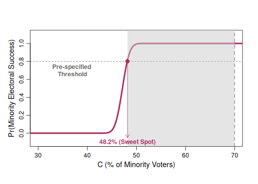
threshold is a probability from 0 to 1. C.prime marks the minority electorate percentage for a district of interest and must be within the plotted range. If it is below the sweet spot, the plot represents a shortfall from the chosen threshold; if it is above, it represents a surplus. Omitting C.prime places it at the calculated sweet spot.

The sweet spot is conditional on the plan and the voting assumptions supplied to sim_redistrict(). It is therefore a comparison tool, rather than a universal electoral threshold.